THE ELEMENTARY AXIOMS OF PROBABILITY (DRAFT)

***** DRAFT *****

This post introduces the basic elements of probability theory, and defines the scope of what I believe should be taught to elementary, or secondary school students. Probability theory is quite simple - simpler than polynomials - but it's one of those things that takes many years to learn. If we are to be able to teach the next stage of AI at a tertiary or undergraduate university level, then we need students to be entering into their first year of university in such a way that they are already familiar with the elementary school level axioms and theorems presented here.

The target audience for this post is those with at least year 10 high-school/elementary level training in algebra, basic probabilities and very basic set-builder notation, and with the ability to Google around for some info on a few new symbols: element of a set $\color{white}\in$, implication $\color{white}\rightarrow$, summation $\color{white}\sum$, infinite limits $\color{white}\lim_{c \to \infty}$, the existential quantifier 'for-all' $\color{white}\forall$, and the empty set $\color{white}\{\varnothing\}$.

This page is incomplete, and is a preview into a forthcoming paper on the elementary axioms of probability. A todo list is provided in the comments. 

Lets begin.

Fair Odds & Jacko's Paradox

We start our journey into the elementary axioms of probability with a familiar concept: gambling, in particular odds. Lets use odds to prove that there is no such thing as absolute certainty, and illustrate how one can use probability theory to derive and prove things.

Direct Proof: Show with absolute certainty, that there is no such thing as absolute certainty.

First we define as an assumption how one converts between odds $\color{white}O(x)$ and probability $\color{white}P(x)$:

$\begin{align*} O(X) = & \frac{P(X)}{1-P(X)} \\ \\ P(X) = & \frac{O(X)}{1+O(X)} \end{align*}$

(in logic, we call these premises)

NB: In the above, the odds function $\color{white}O()$ should not be confused with Knuth's Big-O function $\color{white}\mathcal{O}()$.

You can play with the above two formulas using this spreadsheet to convince yourself analytically and anecdotally that they are correct:

20230226-odds-vs-probabilities.xlsx

Theorem: Now we present as a theorem the proposition that in the limit, as the probability of some event $\color{white}x \in X$ occuring approaches 1.0 or 100% (aka., certainty), the odds of event $\color{white}~x~$ occuring approaches infinity $\color{white}\infty$:

$\begin{align*}\lim_{P(X=x) \to 1.0} O(X=x) = \infty \end{align*}$

(in logic, we call this a proposition)

Derivation: Then we use our previous assumptions to derive a singularity and prove that the theorem is true:

$\begin{align*} P(\texttt{certainty}) = & ~ 1.0 \\ O(\texttt{certainty}) = & ~ \frac{P(\texttt{certainty})}{1 - P(\texttt{certainty})} \\ = & ~ \frac{1}{1-1} \\ = & ~ \frac{1}{0} \\ = & ~ \infty \end{align*}$

(in logic, we call this a proof of our proposition, grounded on the assumed premises)

Summary: From the above, we can now easilly conclude that the odds of absolute certainty is a singularity $\color{white}\infty$, which is not a possibility in reality. The paradox of the above proof is thus: we have just proven, with absolute certainty, that there is no such thing as absolute certainty!

If one is a good neat theoretical computer scientist, then when writing a rigorous math proof, one should close their summary with a description of what has been proved using set-builder notation, as follows:

Id. est:

$\begin{align*} \{ \underset{X \in \textsf{all~random~variables}}{\forall}, x \in X : x {\rm ~is~a~possibility,~} O(X=x) = \infty, P(X=x) = 1.0\} = \{ \varnothing \} \end{align*}$

(set builder is a uni-dimensional notation system for documenting high dimensional set-theoretic things. Note that in place of the usual $|$ notation, we have used $:$ to mean 'such-that' - probabilists keep the former for 'conditioning', so we use the latter colon instead when writing set-builder notation)

As a final step, we close off the proof with a solid square to indicate that this particularly rigorous demonstration has concluded:

$\color{white}\blacksquare$

Discussion: As they say on Wall St, there's no such thing as a free lunch, or at the track, there's no such thing as a sure fire bet! Probability theory is an amazing calculus. With a small handful of elemental axioms, one can do all sorts or extrordiary things, both in a theoretical, mathematical world, and in real life through things such as AI and machine learning. For example, we just used it to prove mathematically (with absolute certainty) three seemingly unrelated concepts are impossible: free Wall St lunches, guaranteed horse tips and absolute certainty. Welcome to the power of probabilistic reasoning!

Let's continue.

Deriving Bayes' Axioms

Grounded on our now established understanding of what probability and certainty is (and with it neatly framed in terms of odds), lets proceed to derive all the elementary probabilistic axioms right through to Bayes Rule and basic conditional independance assumptions.

Derivation: Lets algebraically derive and label the elementary axioms of probability through a sequential sequence of easily understandable steps.

$\begin{align*} & ~ P(A), ~ P(B) & \textsf{\small marginal probabilities} \\ & ~ P(A,B) & \textsf{\small joint probability} \\ P(A,B) = & ~ P(A) \cdot P(B) & \textsf{\small independence} \\ \rightarrow & ~ A \perp B & \textsf{\small independence notation} \\ \rightarrow P(A) = & ~ P(A|B), ~ P(B) = ~ P(B|A) \\ P(A,B) \neq & ~ P(A) \cdot P(B) & \therefore \textsf{\small not independant} \\ P(\neg A) = & ~ P(\bar{A}) & \textsf{\small converse} \\ = & ~ 1 - P(A) \\ \rightarrow 1 = & ~ \sum_{a \in \{A,\bar{A}\}} P(a) & \textsf{\small total probability}\\ P(A|B) = & ~ P(\texttt{cause}~A|\texttt{effect}~B) & \textsf{\small diagnostic reasoning} \\ = & ~ \frac{P(A,B)}{P(B)} & \textsf{\small\emph (explaination)} \\ \rightarrow P(B|A) = & ~ P(\texttt{effect}~B|\texttt{cause}~A) & \textsf{\small causal reasoning} \\ = & ~ \frac{P(A,B)}{P(A)} & \textsf{\small\emph (prediction)} \\ = & ~ \frac{P(\bar{A},B)}{P(\bar{A})} & \textsf{\small counterfactual} \end{align*}$

OK we have now defined causality in terms of two random variables $\color{white}A$ & $\color{white}B$, and introduced the conditioning bar $\color{white}|$. Let's continue:

$\begin{align*} P(A,B) = & ~ P(B|A) \cdot P(A) & \textsf{\small product rule} \\ = & ~ P(A|B) \cdot P(B) \\ \rightarrow P(\bar{A},B) = & ~ P(B|\bar{A}) \cdot P(\bar{A}) & \textsf{\small causal inference} \\ = & ~ P(\bar{A}|B) \cdot P(B) \\ P(B) = & ~ \sum_{a \in A} P(a, B) & \textsf{\small marginalisation} \\ = & ~ P(A,B) + P(\bar{A}, B) \\ = & ~ P(B|A) \cdot P(A) + P(B|\bar{A}) \cdot P(\bar{A}) \end{align*}$

We've now derived the basic components we need to further derive the magical Bayes Rule. Let's do it:

$\begin{align*} P(A|B) = & ~ \frac{P(A,B)}{P(B)} \\ = & ~ \frac{P(B|A) \cdot P(A)}{P(B|A) \cdot P(A) + P(B|\bar{A}) \cdot P(\bar{A})} \\ = & ~ \frac{P(B|A) \cdot P(A)}{P(B)} \\ = & ~ \frac{P(B|A)}{P(B)} \cdot P(A) & \textsf{\small bayes rule (1)}\end{align*}$

Alright, the next part builds on Bayes Rule to introduce two important probabilistic operations: conditioning and normalisation:

$\begin{align*} P(A|B=b) = & ~ \frac{P(A,B=b)}{\sum\limits_{a \in A}P(A=a,B=b)} & ~A~\textsf{\small conditioned on}~b \\ P(A|B) = & ~ \underset{b \in B}{\forall} P(A|B=b) & ~A~\textsf{\small conditioned on}~B \\ P(A|B) \propto & ~ \alpha \cdot P(B|A) \cdot P(A) & \textsf{\small normalization} \\ {\rm where} ~ \alpha = & ~ 1 / \sum_{a \in A} P(B,a) \\ = & ~ 1 / \sum_{a \in A} P(B|a) \cdot P(a) \\ = & ~ {\rm the~'normalization~constant'} \\ \end{align*}$

Note that with $\color{white}A~\textsf{\small conditioned on}~b$ in the above, we have taken the joint probability and created a conditional probability distribution from it. This is a useful tool.

Finally, we have the basic laws of expectation:

$\begin{align*} \omit\rlap{The \textsf{expectation} E[] of a discrete random variable X is:} \\ E[X] = & ~ \sum_{i=1}^{I} x_i \cdot P(X=x_i) & \textsf{\small expectation} \\ \\ \omit\rlap{The \textsf{expectation} of two discrete random variables X + Y is:} \\ E[X+Y] = E[X,Y] = & ~ \sum_{i=1}^{I} \sum_{j=1}^{J} x_i \cdot y_j \cdot P(X=x_y, Y=y_j) & \textsf{\small joint expectation} \\ = & ~ E[X] + E[Y] \\ \\ \omit\rlap{The \textsf{expectation} of X given that Y=y is:} \\ E[X|Y=y] = & ~ \sum_{j=1}^{J} x_j \cdot P(X=x_j|Y=y) & \textsf{\small conditional expectation} \\ \\ \omit\rlap{Sometimes one is interested in some function f() of a random variable X.} \\ \omit\rlap{Thinking of f(X) as your \textsf{payoff function}:} \\ E[\mathnormal{f}(X)] = & ~ \sum_{i=1}^{I} \mathnormal{f}(x_i) \cdot P(X=x_i) & \textsf{\small expected payoff} \end{align*}$

Note that the $\color{white}\textsf{expectation~} E[X]$ may also be referred to as the average, mean or probability weighted average of $\color{white}X$, whilst the $\color{white}\textsf{expected payoff~} E[\mathnormal{f}(X)]$ may sometimes also be referred to as the expected value.

There. All the elementary probabilistic axioms, in one place. I.e., the minimal, or necessary, sufficient and complete set of elemental axioms required to talk about anything to do with probability theory that doesn't involve the very Bayesian concepts of The Chain Rule for Bayesian Networks, or The Markov Condition. We have also avoided joint-probability distributions, for now.

We close off this derivation with the less rigorous:

$\color{white}\textsf{QED}$

Discussion of $\color{white}\textsf{QED}$: this is a reference to the latin phrase "Quod Erat Demonstrandum", which in academic texts is said to mean I have finished my demonstration. I have a different view of latin, and based on my Italian heritage, I think of it more as meaning 'there, I have shown you something'. Either way, one tends to use QED when they are being less formal or rigorous in their description of something, such that the square box would be inappropriate. I tend to use QED quite a lot, because I'm a probabilist rather than a logician, so I sometimes have a more loose view of what it means to prove something, as I don't mind a little uncertainty. Also, according to contemporary vernacular, $\color{white}\textsf{QED}$ means 'look, I did a thing!'

Illustrating the elements of Bayes Rule with a classic example

I now offer you a classic exemplar of applying Bayes Rule - what is the probability that one might have covid virus (V), conditioned on the observed evidence that one has a cough (C)! Lets do it.

$\begin{align*} & {\rm For~the~purposes~of~this~illustration,~} V {\rm ~and~} C {\rm ~are~binary~random~variables.} \\ & {\rm E.g.,~} v \in V {\rm ~is~covid~virus,~} c \in C {\rm ~is~a~cough:}\end{align*}$

And the example that illustrates this concept is as follows:

$\begin{align*} P(A|B) = & ~ \frac{P(B|A)}{P(B)} \cdot P(A) \\ \\ \rightarrow ~ \underbrace{P(\texttt{cause}~A|\texttt{effect}~B)}_{\rm posterior~of~cause} = & ~ \frac{\overbrace{P(\texttt{effect}~B|\texttt{cause}~A)}^{\rm evidence/likelihood}}{\underbrace{P(\texttt{effect}~B)}_{\rm prior~of~effect}} \cdot \underbrace{P(\texttt{cause}~A)}_{\rm prior~of~cause} \\ \\ \rightarrow P(v|c) = & ~ \frac{P(c|v)}{P(c)} \cdot P(v) \\ \\ = & ~ \frac{0.72}{0.05} \cdot 0.013 = 0.1872 \\ \end{align*}$

Now, what we can see from the above is thus:

• $\color{white}P(v):$ There is a 1.30% chance (or 0.013 probability) that anyone might have the covid virus (our prior V).
• $\color{white}P(c):$ There is also a 5% chance (or 0.05 probability) that one might have a cough (regardless of any covid virus). This is the prior probability of observing the evidence we have at hand (ie, a cough).
• $\color{white}P(c|v):$ There is also a 72% chance (or 0.72 probability) that one will have a cough IF THEY HAVE COVID VIRUS. This is the likelihood of observing our evidence (a cough) conditioned on our model (of the things that are causally related to covid virus).
• $\color{white}P(v|c):$ Swizzle all that together, and the probability one has covid virus ( $\color{white}V=true {\rm ~ or ~ just~ } v$) conditioned on observing their cough ( $\color{white}C=true {\rm ~ or ~ just~ } c$) goes from 0.013 (1.30%) to 0.1872 (18.72%).

Got it? If you did, then fabulous, because you just did a Bayesian update!

$\color{white}\textsf{QED}$

Bayesian update worked example

Whilst I am a theorist, my core computer science training was in an officially 'applied' Univerisity (RMIT). At RMIT Univeristy, we always believe that it's important to provide at least one worked example of a theoretical algorithm in action, so that one can analyse it on paper - or in this case, Excel. If one is a properly rigorous 'neat' computer scientist, then they not only present the theory, but they provide worked examples of their theory being appleid in the real world. If an algorithm has particualrly thorny steps, then code snippets rather than pseudo code is the way to go. A good proof of a theorem is not complete if it doesn't have a few $\color{white}\textsf{QED}s$, a worked example and optionally some code snippets.

To fully specify some algorithmic gem:

• The theoretical basis, with rigorous proof(s) and/or set-builder is strongly advised,
• augmented with $\color{white}QED$ examples of edge/corner/extension/related cases, and
• with implementation of worked examples both on paper and optionally in code

is considered a full and complete description of an algorithm. If someone is not rigorous enough to provide each of these elemental components to describe a theoretical whole, then one must ask: do they really know what they're talking about?

Following on from this definition of proper rigour, in the following Excel spreadsheet we calculate the above bayesian update using two methods: directly using point estimates, and through integration of binomial distributions. A little note for elementary students: in the Excel, we have discretised the continuous domain into 'discrete chunks', so you don't have to deal with the integrand symbol $\color{white}\int$ and the mind bending concept of infinitesimals, but rather the more simple repetitive application of addition through summation $\color{white}\sum$. I know it's a jump, but you'll get it in time.

Summation is simply repetitive adding over a set of similar things, for example, adding together the prices of each item you might buy from the school lunch shop. When we discretise, we 'chunk-up' the number line into discrete intervals and estimate the integrand for each interval. Using summation in place of integration will give you an approximate answer but is much easier to understand and compute (actually, this is generally how computers do integration when a programmer hasn't coded-in a formula to calculate an exact answer), whereas if we were to use the integrand and 'integrate over the integral', we would get an exact answer. Keep this in mind when looking at the following spreadsheet, and remember - we're doing integral estimation using discrete summation, and if we want a more accurate estimate or approximation, we could discretise the number line into more discrete intervals (which requires more computations):

20230207-simple-bayesian-update-example.xlsx simple bayesian update example using conjugation

The chart from the Excel example showing the prior $\color{white}P(covid) = 1.30\%$ and
an estimate of the posterior $\color{white}P(covid|cough=true) = 18.78\%$

$\color{white}\textsf{QED}$

Independence of Multiple Events

We are nearly there. The last part of the derivation is to introduce a third random variable $\color{white}C$, define evidential reasoning, then use that to derive a higher order 3-variable Bayes Rule, and the extremely important concept of conditional independence, which we then use to derive a conditional version of the product rule.

Sometimes the independence of two events, $\color{white}A ~ \& ~ B$ is conditional on a third event, $\color{white}C$, i.e.:

$\begin{align*}P(A,B|C) = & ~ P(A|C) \cdot P(B|C)\end{align*}$

but, unlike $\color{white}\textsf{joint probability}$:

$\begin{align*} P(A,B|\bar{C}) \neq & ~ P(A|\bar{C}) \cdot P(B|\bar{C}) \end{align*}$

Extending to $\color{white}>~2$ events: The $\color{white}k$ events $\color{white}A_1, A_2, \cdots, A_k$ are said to be $\color{white}\textsf{mututally independent}$ if for all possible combinations from the set of $\color{white}k$ events, the joint probability is equal to the marginal probabilities.

E.g.: Three events $\color{white}A_1, A_2, A_3$ are mututally independent IFF (note the powerset):

$\begin{align*} P(A_1,A_2) = & ~ P(A_1) \cdot P(A_2) \\ P(A_1,A_3) = & ~ P(A_1) \cdot P(A_3) \\ P(A_2,A_3) = & ~ P(A_2) \cdot P(A_3) \\ P(A_1,A_2,A_3) = & ~ P(A_1) \cdot P(A_2) \cdot P(A_3) \end{align*}$

If any of the above do not hold, then a conditional independence might be entailed in the model. For example, if the first three are satisfied but not the fourth, then the events are said to be $\color{white}\textsf{pairwise independent}$.

More generally:

$\begin{align*} P(A|B,C) = & ~ \frac{P(A,B,C)}{P(B,C)} & \textsf{\small evidential reasoning (prediction)} \\ = & ~ \frac{P(B|A,C) \cdot P(A|C)}{P(B|C)} & \emph{\textsf{\small inductive case}} \\ = & ~ \frac{P(C|A,B)}{P(C|B)} \cdot P(A|B) & \textsf{\small bayes rule (2)} \\ P(A,B|C) = & ~ P(A|B,C) \cdot P(B|C) & \textsf{\small conditional product rule} \\= & ~ P(B|A,C) \cdot P(A|C) \\ P(A,B|C) = & ~ P(A|C) \cdot P(B|C) & \textsf{\small conditional independence} \\ \rightarrow P(A|B,C) = & ~ P(A|C) & \textsf{\small independence assumption (3)} \\ \rightarrow P(B|A,C) = & ~ P(B|C) & \textsf{\small independence assumption (4)} \\ P(A,B|C) = & ~ P(A|B,C) \cdot P(B|C) & \textsf{\small conditional product rule} \\ = & ~ P(B|A,C) \cdot P(A|C) \\ \end{align*}$

The two independence assumptions are easily proven using Bayes Rule, as follows.

Direct proof of (3): Show that $\color{white}P(A|B,C) = P(A|C)$ by deriving it from $\color{white}P(A,B|C)$:

$\begin{align*} P(A,B|C) = & ~ P(A|C) \cdot P(B|C) \\ \rightarrow \frac{P(A,B,C)}{P(C)} = & ~ \frac{P(A,C)}{P(C)} \cdot \frac{P(B,C)}{P(C)} \\ \rightarrow \frac{P(A,B,C)}{\bcancel{P(C)}} \cdot \frac{\bcancel{P(C)}}{P(B,C)} = & ~ \frac{P(A,C)}{P(C)} \cdot \frac{\bcancel{P(B,C)}}{\bcancel{P(C)}} \cdot \frac{\bcancel{P(C)}}{\bcancel{P(B,C)}} \\ \rightarrow \frac{P(A,B,C)}{P(B,C)} = & ~ \frac{P(A,C)}{P(C)} \\ \rightarrow P(A|B,C) = & ~ P(A|C) & \square \\ \end{align*}$

Direct proof of (4): Show that $\color{white}P(B|A,C) = P(B|C)$ by deriving it from $\color{white}P(A,B|C)$:

$\begin{align*} P(A,B|C) = & ~ P(A|C) \cdot P(B|C) \\ \rightarrow \frac{P(A,B,C)}{P(C)} = & ~ \frac{P(A,C)}{P(C)} \cdot \frac{P(B,C)}{P(C)} \\ \rightarrow \frac{P(A,B,C)}{\bcancel{P(C)}} \cdot \frac{\bcancel{P(C)}}{P(A,C)} = & ~ \frac{\bcancel{P(A,C)}}{P(C)} \cdot \frac{P(B,C)}{\bcancel{P(C)}} \cdot \frac{\bcancel{P(C)}}{\bcancel{P(A,C)}} \\ \rightarrow \frac{P(A,B,C)}{P(A,C)} = & ~ \frac{P(B,C)}{P(C)} \\ \rightarrow P(B|A,C) = & ~ P(B|C) & \square \\ \end{align*}$

Note in the above another end-of-proof symbol: this time it's the open square $\color{white}\square$. This means it's a rigorous proof/derivation/whatever, but it is provided merely as an example, illustration or definition (which usually forms part of a bigger $\color{white}\blacksquare$ or $\color{white}\textsf{QED}$).

When a probabilistic model - no matter how small or large - contains independence assumptions, we say that these independendices are entailed in the model, and use special notation to describe all the possible independence assumptions associated with a single conditional independence statement, as follows:

Independence of random variables:

If the random variables $A$ and $B$ are $\textsf{probabilistically independent}$ then we can write:

$\begin{align*} A \perp B \end{align*}$

Furthermore, we can say:

$\begin{align*} A ~ {\rm is ~ irrelevant ~ to} ~ B \end{align*}$

Conditional independence of random variables:

If the random variables $A$ and $B$ are $\textsf{conditionally independent}$ given the random variable $C$, then we can write:

$\begin{align*} A \perp B ~ | ~ C \end{align*}$

To mean:

$\begin{align*} A ~ {\rm is ~ irrelevant ~ to} ~ B ~ {\rm given} ~ C\end{align*}$

This is much easier notation than listing out every entailed independence assumption as per the examples provided in the Direct Proofs of (3) & (4) above.

NB: Independence is a modelling assumption.

Extending to $\color{white}>~3$ events:

To extend the generalised (not-Bayesian) probabilistic calculus to more than 3 events or random variables, one applies the generalised Product Rule. It's provided here just for completeness, and doesn't need to be understood for the purposes of this article - just that it exists:

$\begin{align*} P(\vec{X}) = & ~ P(X_1, \cdots, X_n) \\ = & ~ P(X_n|X_{n-1},\cdots,X_1) \cdot P(X_{n-1}|X_{n-2},\cdots,X_1) \cdots P(X_2|X_1) \cdot P(X_1) \\ = & ~ \prod_{i=1}^{n}P(X_i|X_{i-1},\cdots,x_1) \end{align*}$

E.g.:

$\begin{align*} P(A,B,C,D) = & ~ P(A|B,C,D) \cdot P(B|C,D) \cdot P(C|D) \cdot P(D) \\ = & ~ P(D|C,B,A) \cdot P(C|B,A) \cdot P(B|A) \cdot P(A) \end{align*}$

$\color{white}\textsf{QED}$

Claude Shannon's information theory and entropy

...@TODO

Propensity, probabilistic terminology & notation

A comment on terminology before we close this sequence of demonstrations. In the above we have carefully used a combination of uppercase and lowercase when describing probability as follows:

• uppercase single letters to refer to $\color{white}\textsf{random variables}$, e.g, $\color{white}P(V)$,
• lowercase single letters to refer to $\color{white}\textsf{possibilities}$ associated with $\color{white}\textsf{random variables}$, e.g, $\color{white}P(v)$, which ususally has a $\color{white}probability$ associated with it, and
• lowercase words, which is a more informal and descriptive way of naming a $\color{white}\textsf{random variable}$, e.g, $\color{white}P(covid)$. Consider these a synonym for the uppercase single letter variant, i.e, $\color{white}P(V)$.

Also in probability theory, vernacular or lexicon is important: possibility, likelihood, chance, probability and odds, outcomes and alternatives, mutual exclusivitity and collective exhaustivity, expectation, expected payoff, expected value, utility curve, risk preferences, random variables and 'not too shabby' (amongst others) are all very strictly defined words/phrases in probability theory. I have listed the reserved words here:

• $\color{white}\textsf{decision}:$ An irreversible allocation of resources
• $\color{white}\textsf{probability~} and \textsf{~odds}:$ A measure of uncertainty associated with a possibility.
• $\color{white}\textsf{random variable}:$ a CPD or a CPT specifying a mututally exclusive and collectively exhaustive set of possibities, each with their own associated probabilities.
• $\color{white}\textsf{joint (probability) distribution}:$
• $\color{white}\textsf{possibility}:$
• $\color{white}\textsf{likelihood~} or \textsf{~evidence}:$
• $\color{white}\textsf{chance}:$
• $\color{white}\textsf{uncertainty}:$ a measure of what we don't know
• $\color{white}\textsf{alternatives}:$ possibilities associated with a decision
• $\color{white}\textsf{outcome}:$ the choice from a set of possibilities or alternatives, after a random variable or decision is resolved / observed (respectively).
• $\color{white}\textsf{mutual exclusivity~} and \textsf{~collective exhaustivity}:$ a disjoint set of necessary, sufficient and complete alternatives or possibilities associated with a decision or a random variable (respectively).
• $\color{white}\textsf{expectation}:$ mean. average, mu $\color{white}\mu$ associated with a CDF.
• $\color{white}\textsf{expected payoff}:$
• $\color{white}\textsf{expected value}:$ see expected payoff.
• $\color{white}\textsf{utility curve}:$ a 2-dimensional quantitative assesment of one's risk preferences.
• $\color{white}\textsf{risk preferences}:$ a qualitative assessment of one's appetite for risk, broadly categorised into risk-seeking, risk-neutral or risk averse. Captured in a utility curve.
• $\color{white}\textsf{conditional probability distribution (CPD)}:$
• $\color{white}\textsf{conditional probability table (CPT)}:$
• $\color{white}\textsf{probability mass function (PMF)~} or \textsf{~probability density function (PDF)}:$
• $\color{white}\textsf{cumulative distribution function (CDF)}:$ not relevant.
• $\color{white}\textsf{'not too shabby'}:$ beating a coin flip, or 0.50 probability.
• $\color{white}\textsf{\&}:$ background knowledge of information not captured in a model.
• $\color{white}\textsf{prior probability}:$
• $\color{white}\textsf{posterior probability}:$

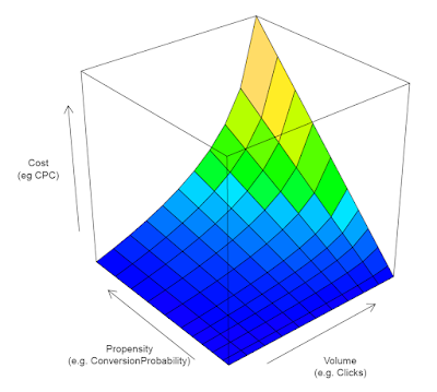
If you are unsure which one to use, or if you are not a probabilist, a frequentist (or a professional gambler!), then I recommend you use the words propensity & utility. I am nowhere near as brutal, but I have attended lectures at NYU where a professor literally stopped a PhD student mid-presentation and said 'You are wasting all our time, get off the stage' just for using the wrong terminology - NYU can be a brutal place, but he did have a point. Be careful not to use these reserverd words unless you know what you're doing. If in dobut, propensity & utility it out.

For an example of using the word propensity, in this chart I produced for a post on digital advertising, the audience is business stakeholders, so I used the word propensity:

Summary and next steps

I hope you enjoyed this very succinct derivation and illustration of Bayes Rule in action. A more detailed paper will be forthcoming in due course that lists out these elementary axioms with properly worked examples. In time, a seccond paper will follow with many more advanced theorems and axioms suitable for a first-year university level student, including Bayesian Networks, the Markov Condition, The Markov Blanket, and various types of inference including direct inference, variable elimination, treeifying and even MCMC.

Understanding all these elemental operations are an important foundation before we can explore Probabilistic Logic. Representing logic with the Bayesian calculus is very interesting: we have classical first and second order logic, third order is fuzzy logic, fourth order is fuzzy set logic and fifth order is magic logic. On this site I will introduce these 5 functional forms in terms of probability theory, then I'll show how they can be treated as Bayesian micro-patterns to build up highly complex tappestries that forms self-determining AI.

For full order Probabilistic Logic to work, the Decision Analysis (DA) calculus with also need a handful of small but significant tweaks. DA hasn't seen any significant changes since the 90s, so I think a bit of a review and a Bayesian update is in order anyhow. Computers are alot bigger and faster these days, so I think it's time to extend it a little. Not much, just a smidge: the thing with all of these probabilistic calculuses is that their elemental componentry is very minimal - but the asssembalages that can be constructed from them are extrordinary.

Please feel free to put any questions in the comments if anything isn't clear enough.

References

...@TODO

.\p

25 February, 2022.